Bitcoin Trade Arrival as Self-Exciting Process
Introduction
This article describes a model that explains the clustered arrival of trades and shows how to apply it to Bitcoin exchange data. This is interesting for many reasons. For example, for trading purposes it is very useful to be able to predict whether there is more buying or selling going on in the short term. On the other hand, such a model might help understand the difference between fundamental news driving the price versus robot traders reacting to price changes.
I show how to fit such a model to MtGox data and also provide all the code and data for it on my Github.
Self-excitability and clustering of order arrivals
Trades do not arrive in evenly spaced intervals but usually arrive clustered in time. This should be clear for anyone who has been watching an orderbook for some time. Similarly, the same trade signs tend to cluster together and result in a sequence of buy or sell orders. Various explanations for this are possible, such as algorithmic traders who split up their orders in smaller blocks or trading systems that react to certain exchange events.
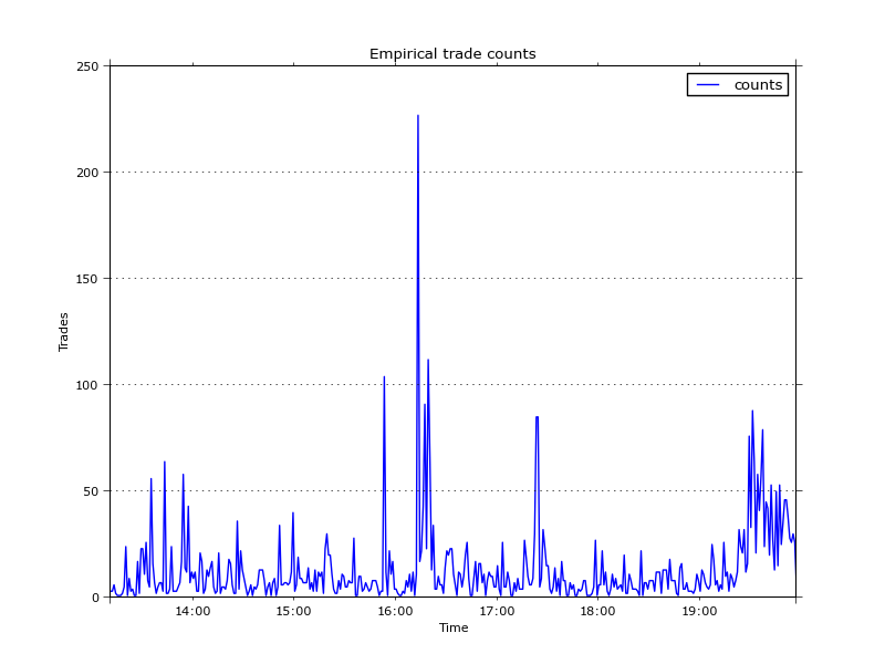
For demonstration purposes, the data I worked with were 5000 trades between 13:10 and 19:57 on the 20 April 2013 (also available on Github). Here is a plot of the trade counts aggregated over a 1 minute window.

The average trade count per minute is 13, however we can make out a couple of instances where it exceeds 50. Usually the higher trade intensity lasts a couple of minutes and then dies down again towards the mean. In particular, the 15 minutes or so after 16:00 we can see very high trading intensity with one instance of over 200 orders per minute, then a slow decrease of intensity over the next ~10 minutes.
The most basic way to describe arrival of event counts, such as the time series above, is a Poisson process with one parameters \(\lambda\). In a Poisson process the expected number of events per unit of time is defined by the one parameter. This method is widely used as it fits well to a lot of data, such as the arrival of telephone calls in a call centre. For our purposes however this is too simple as we need a way to explain the clustering and mean reversion.
Hawkes processes, or also called self-exciting processes, are an extension of the basic Poisson process which aim to explain such clustering. Self-excitable models like this are widely used in various sciences; some examples are seismology (modelling of earthquakes and volcanic eruptions), ecology (wildfire assessment [7]), neuroscience (modelling of brain spike trains which bunch together [6]), even modelling of eruption of violence ([5] on modelling civilian deaths in Iraq, and [8] on crime forecasting), and naturally finance and trading (more to that in a section below).
Let's move on to understanding and fitting a Hawkes process to the data above.
Hawkes Processes
A Hawkes process models the time-varying intensity, or event occurrence rate of a process, which is partially determined by the history of the process. A simple Poisson process on the other hand does not take the history of events into account.
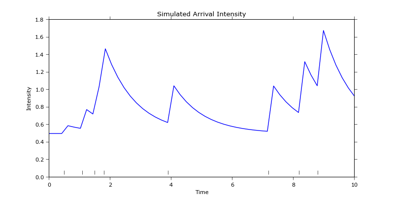
An example realisation of a Hawkes process is plotted in the next figure.

It consists of 8 events, which usually take the form of time stamps, indicated by the rug and a sample intensity path which is defined by three parameters
$$(\alpha, \beta, \mu) = (0.1, 1, 0.5)$$
Here, \(\mu\) is the base rate the process reverts to, \(\alpha\) is the intensity jump right after an event occurrence, and \(\beta\) is the exponential intensity decay. The base rate can also be interpreted as the intensity of exogenous events (to the process) such as news. The other parameters \(\alpha\) and \(\beta\) define the clustering properties of the process. It is usually the case that \(\alpha \lt \beta\) which ensures that the intensity decreases quicker than new events increase it -- otherwise the process could explode.
The self-excitability is visible by the first four events prior to time mark 2. They occur within short time from each other which leads to a large peak of intensity by the fourth event. Every event occurrence increases the chance of another occurrence which results in clustering of events. The fifth data point only arrives at time mark 4 which, in the meantime, resulted in an exponential decrease of the overall intensity.
The conditional intensity takes, in its simplest flavour, the form
$$\lambda(t) = \mu + \sum_{t_i \lt t} \alpha e^{-\beta (t-t_i)}$$
The exponential function defines the memory of the process, i.e. how past events affect the current event. Summation applies this function over the history of events \(t_i\) up to the current event \(t\). \(\lambda(t)\) then represents the instantaneous intensity at time \(t\).
Given the conditional intensity, two derived quantities are also of interest: The expected intensity which (under some conditions) can be shown [4] to have the form
$$E[\lambda] = \frac{\mu}{1- \frac{\alpha}{\beta}}$$
and describes the trading intensity for a given time period. The other quantity is the so called branching ratio
$$n = \int_0^\infty \alpha e^{-\beta t} dt = \frac{\alpha}{\beta}$$
which describes the fraction of trades that are endogenously generated (i.e. as a result of another trade). This can be used to evaluate how much of the trading activity is caused by feedback.
The parameters of the model can be fitted using conventional Maximum Likelihood Estimation and a convex solver. Alternatively, you can use an R package such as ptproc [9], which is what I am going to use in this article.
Fitting Bitcoin Trade Arrival to a Hawkes Process
The intensity path is fully defined given a set of ordered trade times \(t_1 \lt t_2 \lt \cdots \lt t_n\) which, in our case, are just unix timestamps of when the trades were recorded. Given this we can easily apply MLE using the ptproc package. The following function fits the model given an initial guess of the parameters and constraints on the parameters being positive.
fit_hawkes <- function(data) {
  # initial guess where a is alpha and C is beta
  pstart <- c(mu = 0.5, C = 1, a = 0.1)

  # create a ptproc object using the conditional intensity function as defined by ptproc
  ppm <- ptproc(pts = data, cond.int = hawkes.cond.int, params = pstart)

  # assumption that the intensity has to be positive
  condition(ppm) <- penalty(code = NULL, condition = quote(any(params < 0)))

  # fit using standard optim
  f <- ptproc.fit(ppm, optim.control = list(trace = 2), alpha = 1e+5, hessian = TRUE)

  return (f)
}
I ran the fitting procedure above by passing it the 5000 trade timestamps stored in the trade_times dataframe (which I exported from Python). The only difference to the original dataset is that I added a random millisecond timestamp to all trades that share a timestamp with another trade. This is required as the model requires to distinguish every trade (i.e. every trade must have a unique timestamp). The literature describes different ways to address this [4, 10] but extending the timestamps to millisecond is a common one.
> f <- fit_hawkes(trade_times[0:5000])
> summary(f)
Model name: HAWKES.COND.INT

Fitted Parameter Values:
            mu               C               a
0.070223167168  1.795900246884  1.182079921093

Model AIC:  13788.389497822
H. Pois. AIC:  25836.993184719
We end up with the parameter estimates of \(\mu = 0.07, \alpha = 1.18, \beta = 1.79\). The parameter estimate of \(\alpha\) shows that right after a single trade occurs, the conditional intensity increases by 1.18 trades per second. Further, the average intensity over the whole period is \(E[\lambda] = 0.20\) trades per second, over a minute adding up to 12 trades, which matches our empirical counts. The branching ratio of \(n = 65\%\) indicates that more than half of the trades are generated within the model as a result of other trades. This is high given that the hours studied are relatively quiet with the price trending upwards. It would be interesting to apply this to more turbulent regimes (e.g. some of the crashes) where I assume the ratio will be much higher.
The aim is now to compute the actual conditional intensity for the fitted model and compare it against the empirical counts. The R package contains a function evalCIF to do this evaluation, we only have to provide a range of timestamps to evaluate it at. This range is between the min and max timestamp of the original data set, for every point within the range the instantaneous intensity is calculated.
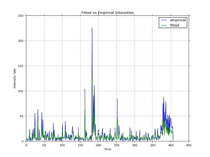
This leads to the following plot comparing empirical counts (from the first plot of this article) and the fitted, integrated intensities.

Purely visually, it appears to be quite a good fit. Notice that the historical intensities are often above the fitted ones, which has already been observed in [12] (in the appendix). The authors addressed this by introducing influential and non-influential trades, which effectively reduces the number of trades which are part of the fitting procedure. Another reason for this slight mismatch in jump sizes between empirical and fitted data could be the randomisation of timestamps within the same second; over 2700 out of the 5000 original trades share a timestamp with another trade. This results in a lot of trades (within the same second) losing their order, which could influence the jump sizes.
The effect of timestamp randomisation has been studied in [10].
Goodness of Fit
There are many ways of evaluating the goodness of fit. One is by comparing AIC values against a homogenous Poisson model which shows, as visible in the R summary above, that our Hawkes model is a considerably better fit for the data.
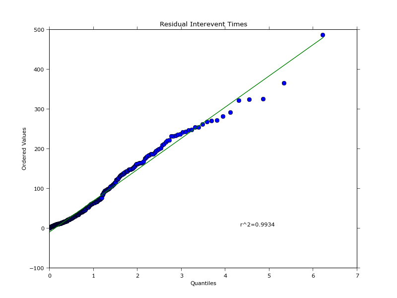
Another way to test how well the model fits the data is by evaluating the residuals (which are kind of hard to obtain for a Hawkes process, thankfully ptproc does the job). Theory says [4] if the model is a good fit, then the residual process should be homogenous and should have interevent times (the difference between two residual event timestamps) which are exponentially distributed. A log-survivor plot of the interevent times (as suggested by [9]), or equally in our case a QQ-plot against an exponential distribution, confirms this. The plot below shows an excellent R2 fit.

Now that we know the model explains clustering of arrivals well, how can this be applied to trading? The next steps would be to at least consider buy and sell arrivals individually and find a way to make predictions given a fitted Hawkes model. These intensity predictions can then form a part of a market-making or directional strategy. Let us have a look at the literature to get some ideas.
Application to Trading
The paper in [4] describes very clearly how to fit and evaluate Hawkes processes in a financial setting. Florenzen also treats the different ways of disambiguating multiple trades in the same timestamp and evaluates the result on TAQ data.
Hewlett [2] predicts the future imbalance of buy and sell trades using a bivariate self- and cross-excitation process between buy and sell arrivals. The author devises an optimal liquidation strategy, derived from a price impact formula based on this imbalance.
In [3] the authors use the buy and sell intensity ratio of a bivariate Hawkes process as an entry signal to place a directional trade.
In [12] the authors develop a high frequency market-making strategy which distinguishes between influential and non-influential trades as a way to get a better fit of their Hawkes model to the data (I assume). A further ingredient in the model is a short-term midprice drift which allows placement of directional bets and avoids some adverse selection. Their placement of bid and ask quotes then depends on the combination of the short-term drift, order imbalance (asymmetric arrivals of buy and sell), and inventory mean reversion.
Improvements
The loglikelihood function of a Hawkes process has a computational complexity of O( N2 ) as it performs nested loops through the history of trades. This is very expensive and leads to a fitting time of 12 minutes for 5000 trades on my Macbook pro. There is a recursive formulation of the likelihood which memoises the calls and speeds up evaluation [10]. This is still inefficient, especially for high-frequency trading purposes where fast fitting procedures are a primary interest.
While it is not quite clear what is actually used by HFT practitioners, some recent research from this year demonstrates how to calculate intensity rates using GPUs [11]. This clearly indicates that there is interest in very fast Hawkes calibration.
Some even more recent research [1], published last month, by Fonseca and Zaatour, describes fast calibration without evaluating the likelihood function. Instead, the authors use Generalised Method of Moments to estimate the parameter values. They show how to compute, in closed-form, moments of any order and autocorrelation of the number of jumps within a given time interval. While not as accurate as MLE, the GMM seems to provide an "immediate" (in the words of the authors) estimation. No comparison in speeds is provided but from what I understood all that is required is to calculate the empirical autocorrelation over a number of time lags and to minimise the objective function.
Conclusion
In this article I showed that a Hawkes process is a good model for explaining the clustered arrival of Mtgox trades. I showed how to estimate and evaluate a model given trade timestamps and highlighted some of the issues around estimation.
Bitcoin exchange data and its price discovery has not been studied well (or at all?) yet. Self-exciting models might answer questions such as how much of Bitcoin price movements are due to fundamental events, or how much is a result of lots of reactionary algorithms hooked up on Mtgox's API. The model itself could naturally be also part of a trading strategy.
You can get the data and code to reproduce the graphs and results from this repository.
References
[1] J. Fonseca, and R. Zaatour: Hawkes Process: Fast Calibration, Application to Trade Clustering and Diffusive Limit ssrn.
[2] P. Hewlett: Clustering of order arrivals, price impact and trade path optimisation pdf.
[3] J. Carlsson, M. Foo, H. Lee, H. Shek: High Frequency Trade Prediction with Bivariate Hawkes Process.
[4] F. Lorenzen: Analysis of Order Clustering Using High Frequency Data: A Point Process Approach pdf.
[5] E. Lewis, G. Mohler, P. Brantingham, and A. Bertozzi: Self-Exciting Point Process Models of Civilian Deaths in Iraq pdf.
[6] P. Reynaud-Bouret, C. Tuleau-Malot, V, Rivoirard, and F. Grammont: Spike trains as (in)homogeneous Poisson processes or Hawkes processes: non-parametric adaptive estimation and goodness-of-fit tests pdf.
[7] R.D. Peng: Applications of Multi-dimensional Point Process Methodology to Wildfire Hazard Assessment.
[8] G.O. Mohler, M.B. Short, P.J. Brantingham, F.P. Schoenberg, and G.E. Tita: Self-Exciting Point Process Modeling of Crime pdf.
[9] R.D. Peng: Multi-dimensional Point Process Models in R pdf.
[10] V. Filimonov, and D. Sornette: Apparent criticality and calibration issues in the Hawkes self-excited point process model: application to high-frequency financial data arxiv.
[11] C. Guo and W. Luk, E. Vinkovskaya, and R. Cont: Customisable Pipelined Engine for Intensity Evaluation in Multivariate Hawkes Point Processes pdf.
[12] A. Cartea, S. Jaimungal, and J. Ricci: Buy Low Sell High: A High Frequency Trading Perspective ssrn.
comments powered by Disqus